Position-Time Graphs - Complete Toolkit
Objectives
-
To relate the shape (horizontal line, diagonal line, downward-sloping line, curved line) of a position-time graph to the motion of an object.
-
To relate the slope value of the line on a position-time graph at a given time or during a given period of time to the instantaneous or the average velocity of an object.
-
To use a slope calculation to find the instantaneous or average velocity of an object.
-
To relate the motion of an object as described by a position-time graph to other representations of an object's motion - dot diagrams, motion diagrams, tabular data, etc.
Readings from The Physics Classroom Tutorial
-
The Physics Classroom Tutorial, 1D-Kinematics Chapter, Lesson 3
http://www.physicsclassroom.com/class/1DKin/U1l3a.html
Interactive Simulations
-
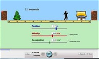
PhET Simulation: The Moving Man
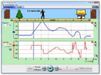 This interactive simulation lets learners move a little man on the screen and view the resulting graphs of position, velocity, and acceleration. It was developed to help beginners explore why the graphs follow predictable patterns. Set initial conditions and view the graphs simultaneously as the "Moving Man" changes position. You can also program the motion by entering an equation for the position as a function of time and play it back in slow motion or at real speed. Note: For introductory explorations, you can “uncheck” the Acceleration vs. Time graph.
-
PhET Supplementary Materials: The Moving Man
 Inquiry-based materials developed by the PhET team specifically for use with The Moving Man. This one includes Power Point concept questions (with answers provided), lesson plan, pre-lab and post-lab assessments, and printable student guidelines. You can parse out materials related to Position vs. Time graphs in introducing your kinematics unit. The simulation allows you to display any of the three motion graphs individually or view all three simultaneously.
-
Concord Consortium: Describing Velocity
 This classroom-tested graphing activity explores similarities and differences between Position vs. Time and Velocity vs. Time graphs. It accepts user inputs in creating prediction graphs, then generates an accurate comparison graph for the process being analyzed. Learners will annotate graphs to explain changes in motion, respond to question sets, and analyze why the two types of graphs appear as they do. Note: Although it’s designated for Grades 6-9, this activity is robust enough to use as an introduction to motion graphing for high school physics.
Video and Animations
-
Physlet Physics: Average Velocity
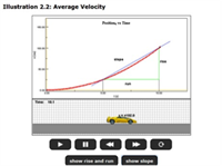 This animation shows the Position vs. Time graph for a car traveling at non-constant velocity. Students can view “Rise and Run” to see that the rise is the displacement and run is the time interval. Click “Show Slope” to see how the slope of the line represents the average velocity. Simple, but packs punch.
-
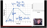
Position vs. Time and Velocity vs. Time Graphing
 For students who continue to struggle with motion graphing after instruction, this video provides help in relating distance traveled and velocity through graph representations. It gives explicit explanations of how to use slope of a P/T graph to determine average velocity, and how to use the area under the curve on a V/T graph to determine the change in position.
-
Bozeman Science: Position vs. Time Graph-Part 1
 For your students with disabilities, English Language Learners, or kids who read below grade level, this video can be a good choice for help in interpreting Position vs. Time graphs. The author is a high school physics teacher from Bozeman, Montana. His easygoing, conversational style keeps it simple, while still introducing the requisite math. This video explores motion of an object with constant velocity.
Labs and Investigations
Minds On Physics Internet Modules:
The Minds On Physics Internet Modules are a collection of interactive questioning modules that target a student’s conceptual understanding. Each question is accompanied by detailed help that addresses the various components of the question.
-
Kinematic Graphing, Assignment KG1 - Basics of p-t Graphs
-
Kinematic Graphing, Assignment KG2 - Interpreting p-t Graphs (I)
-
Kinematic Graphing, Assignment KG3 - Interpreting p-t Graphs (II)
-
Kinematic Graphing, Assignment KG4 - Slope Calculations
Concept Building Exercises:
-
The Curriculum Corner, 1D Kinematics, Describing Motion with Position-Time Graphs
-
The Curriculum Corner, 1D Kinematics, Describing Motion Graphically
-
The Curriculum Corner, 1D Kinematics, Graphing Summary
Problem-Solving Exercises:
-
The Calculator Pad, 1-Dimensional Kinematics, Problems #10 - #12
Science Reasoning Activities:
-
Science Reasoning Center, 1-D Kinematics, Kinematics
Related PER (Physics Education Research)
-
Kinematics Graph Interpretation Project
Recent work has uncovered a consistent set of student difficulties with graphs of position, velocity, and acceleration vs. time. For the busy teacher, this synopsis will be a quick read but worth every minute. It organizes the findings of several years of the Kinematics Graph Interpretation Project on one page.
-
Searching for Evidence of Student Understanding, T. Bartiromo, presented at the Physics Education Research Conference 2010, Portland, Oregon
This research examined whether high school students can translate between representations (an ability often considered to be an “expert trait” in solving physics problems). It also gauged whether requiring multiple representations for a single problem helped instructors better assess student understanding. It’s a short read (3.5 pages), and has interesting implications: “We can argue that by assessing students with multiple choice questions or by requiring only one representation, one might get a false sense of students’ mastery…..Therefore, assessments need to include problems in which students respond with more than one representation.”
Common Misconceptions:
-
Slowing Down vs. Downward Slopes
A common student difficulty pertains to mistaking a slowing down motion for a line that slopes downward on a position-time graph. The slope of a line represents the velocity of an object. An object that slows down is described by a line with a decreasing slope. Whether the slope itself is positive (upward) or negative (downward) is of little importance in determining if the speed is increasing or decreasing. The source of this student difficulty may be in the dual use of the word down: slowing down and sloping down. As such, it may be better to use the phrase getting slower in place of the phrase slowing down.
-
Negative and Positive Acceleration
Students are often troubled by the concept of a negative acceleration. In physics, positive and negative signs associated with quantities have physical meaning. In the case of acceleration, a positive and negative indicate directional information. An object with a negative acceleration is not necessarily slowing down. Objects that are slowing down simply have an acceleration value that is opposite of the direction of their velocity value. So if an object is moving in the positive direction and slowing down, it has a negative acceleration. But if an object is moving in the negative direction and slowing down, it has a positive acceleration. Conversely, if an object is moving in the negative direction and speeding up, it has a negative acceleration. When translating this information to position-time graphs, a negative acceleration could be represented by an upward sloping line that becomes flatter with time or a downward sloping line that gets steeper with time.
-
Slope Calculations
Some students can have difficulty with slope calculations. Most difficulties are associated with implementing an erroneous method. The slope of a line is a ratio of the change in y-coordinate to change in x-coordinate for any two points located on the line. For a line that passes through the origin, the calculation naturally simplifies to the ratio of the y-coordinate to the x-coordinate for any single point on the line. But this simplification has a clear condition attached - "for a line that passes through the origin."
PER-Based Experiment:
-
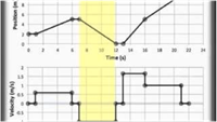
Catching Mistakes: The Case of Motion Graphs
 This classroom experiment was developed as an outgrowth of PER (Physics Education Research). Students are encouraged to explore and actively learn from their mistakes, using an instructional method developed by the University of Maryland PER Group. First, learners predict the appearance of position and velocity graphs for different types of walking motion, then verify their predictions with a motion sensor. If all members of the group predict correctly, they move on. If not, the group’s task is to analyze the error, figure out what went wrong, then write statements about how to modify incorrect ideas. Allow one class period.
Standards:
A. Next Generation Science Standards (NGSS)
Note: The topic of kinematics is not directly covered in the NGSS.
B. Common Core Standards for Mathematics – Grades 9-12
Standards for Mathematical Practice
-
MP.2 Reason abstractly and quantitatively
-
MP.6 Attend to precision
-
MP.8 Look for and express regularity in repeated reasoning
Quantities: Reason Quantitatively and Use Units to Solve Problems
-
N-Q.1 Use units as a way to understand problems and to guide the solution of multi-step problems; choose and interpret units consistently in formulas; choose and interpret the scale and the origin in graphs and data displays.
-
N-Q.3 Choose a level of accuracy appropriate to limitations on measurement when reporting quantities.
Algebra: Seeing Structure in Expressions – Interpret the Structure of Expressions
-
A-SSE.1.a Interpret parts of an expression, such as terms, factors, and coefficients
-
A-SSE.2 Use the structure of an expression to identify ways to rewrite it.
Algebra: Creating Equations
-
A-CED.2 Create equations in two or more variables to represent relationships between quantities; graph equations on coordinate axes with labels and scales.
-
A-CED.4 Rearrange formulas to highlight a quantity of interest, using the same reasoning as in solving equations.
Functions: Interpret Functions that Arise in Terms of a Context
-
F-IF.4 For a function that models a relationship between two quantities, interpret key features of graphs and tables in terms of the quantities, and sketch graphs showing key features given a verbal description of the relationship.
-
F-IF.6 Calculate and interpret the average rate of change of a function (presented symbolically or as a table) over a specified interval. Estimate the rate of change from a graph.
Building Functions: Linear, Quadratic, and Exponential Models
-
F-LE.1.b Recognize situations in which one quantity changes at a constant rate per unit interval relative to another.
-
F-LE.1.c Recognize situations in which a quantity grows or decays by a constant percent rate per unit interval relative to another.
Functions: Interpret Expressions for Functions in Terms of the Situation They Model
-
F-LE.5 Interpret the parameters in a linear or exponential function in terms of a context.
Reading Level
This set of tutorials scored 61.84 on the Flesch-Kincaid Readability Index, corresponding with Grade 8. It scored 11.20 on the Gunning-Fog Index, which indicates the number of years of formal education a person requires in order to easily understand the text on the first reading (corresponding to Grade 11).
C. Common Core Standards for English/Language Arts (ELA) – Grades 9-12
Craft and Structure
-
RST.11-12.4 Determine the meaning of symbols, key terms, and other domain-specific words and phrases as they are used in a specific scientific or technical context relevant to grades 11-12 texts and topics.
Integration of Knowledge and Ideas
-
RST.11-12.9 Synthesize information from a range of sources (e.g., texts, experiments, simulations) into a coherent understanding of a process, phenomenon, or concept, resolving conflicting information when possible.
Range of Reading and Level of Text Complexity
-
RST.11.12.10 By the end of grade 12, read and comprehend science/technical texts in the grades 11-CCR text complexity band independently and proficiently.
D. College Ready Physics Standards (Heller and Stewart)
Essential Knowledge-Middle School
Constant and Changing Linear Motion
-
M.3.1.1 The basic patterns of the straight-line motion of objects are: no motion, moving with a constant speed, speeding up, slowing down and changing (reversing) direction of motion. Sometimes an object’s motion can be described as a repetition and/or combination of the basic patterns of motion.
-
M.3.1.2 An object that travels the same distance in each successive unit of time has a constant speed. The constant speed of an object can be represented by and calculated from the mathematical representation (speed = distance traveled/time interval), data tables, a motion diagram, and the slope of the linear distance versus time graph.
-
M.3.1.3 When the distance an object travels increases with each successive unit of time, it is speeding up; when the distance an object travels decreases with each successive unit of time, it is slowing down.
-
M.3.1.4 The relationship between distance and time is nonlinear when an object’s speed is changing and when it is moving in a series with different constant speeds.
-
The constant speed an object would travel to move the same distance in the same total time interval is the average speed.
-
Average speed can be represented and calculated from the mathematical representation (average speed – total distance traveled/total time interval), data tables, and the nonlinear Distance vs. Time graph.
-
For objects traveling to a final destination in a series of different constant speeds, the average speed is not the same as the average of the constant speeds.
Essential Knowledge: High School
Constant and Changing Linear Motion
-
H.3.1.1 The displacement, or change in position, of an object is a vector quantity that can be calculated by subtracting the initial position from the final position, where initial and final positions can have positive and negative values. Displacement is not always equal to the distance traveled.
-
H.3.1.2 An object that travels the same displacement in each successive unit time interval has constant velocity. Constant velocity is a vector quantity and can be represented by and calculated from a position versus time graph, a motion diagram or the mathematical representation for average velocity. The sign (+ or -) of the constant velocity indicates the direction of the velocity vector, which is the direction of motion.
-
H.3.1.3 The constant velocity an object would travel to achieve the same change in position in the same time interval, even when the object’s velocity is changing, is the average velocity for the time interval. Average velocity can be mathematically represented by vave = (xf - xi)/(tf - ti). For straight-line motion, average velocity can be represented by and calculated from the mathematical representation, a curved position versus time graph and a motion diagram.
-
H.3.1.4 The velocity of an object in straight-line motion changes continuously, from instant to instant while it is speeding up or slowing down and/or changing direction. The velocity of an object at any instant (clock reading) is called its instantaneous velocity. The object does not have this velocity over any time interval or travel any distance with this velocity. Instead, the instantaneous velocity is the constant velocity at which an object would continue to move if its motion stopped changing at that instant. An object with zero instantaneous velocity can be accelerating (e.g., motion up a ramp then back down the ramp).
-
H.3.1.5 When the change in an object’s instantaneous velocity is the same in each successive unit time interval, the object has constant acceleration. For straight-line motion, constant acceleration can be represented by and calculated from a linear instantaneous velocity versus time graph, a motion diagram and the mathematical representation [a = (vf - vi)/(tf - ti)]. The sign (+ or -) of the constant acceleration indicates the direction of the change-of-velocity vector. A negative sign does not necessarily mean that the object is traveling in the negative direction or that it is slowing down. [BOUNDARY: The term “deceleration” should be avoided because students tend to associate a negative sign of acceleration only with slowing down.]
Learning Outcomes
-
Represent and calculate the distance traveled by an object, as well as the displacement, the speed and the velocity of an object for different problems. Representations include data tables, distance versus time graphs, position versus time graphs, motion diagrams and their mathematical representations. Interpret the meaning of the sign (+ or -) of the displacement and velocity.
-
Investigate, and make a claim about the straight-line motion of an object in different laboratory situations. Representations include data tables, position versus time graphs, instantaneous velocity versus time graphs, motion diagrams, and their mathematical representations. When appropriate, calculate the constant velocity, average velocity or constant acceleration of the object. Interpret the meaning of the sign of the constant velocity, average velocity or constant acceleration. Interpret the meaning of the average velocity.
-
Explain what is “constant” when an object is moving with a constant velocity and how an object with a negative constant velocity is moving. Justify the explanation by constructing sketches of motion diagrams and using the shape of position and instantaneous velocity versus time graphs.
-
Explain what is “constant” when an object is moving with a constant acceleration and explain the two ways in which an object that has a positive constant acceleration and the two ways in which an object that has a negative constant acceleration. Justify the explanations by constructing sketches of motion diagrams and using the shape of instantaneous velocity versus time graphs.
-
Compare and contrast the following: distance traveled and displacement; speed and velocity; constant velocity and instantaneous velocity; constant velocity and average velocity; and velocity and acceleration.
-
Translate between different representations of the motion of objects: verbal and/or written descriptions, motion diagrams, data tables, graphical representations (position versus time graphs and instantaneous velocity versus time graphs) and mathematical representations.