Calculating Magnetic Flux

Faraday discovered that a changing magnetic field near a coil of wire produces a current in that wire.  This discovery led to an important concept called magnetic flux.  Let’s develop this concept of magnetic flux in this section and then we’ll see how this concept is such an important part of Faraday’s Law  in the next section.

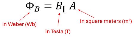
Magnetic flux is quantity that measures the magnetic field passing through an area.  Physicists use the symbol Φ_B for magnetic flux.  We’ll find two equivalent expressions for magnetic flux to be helpful:

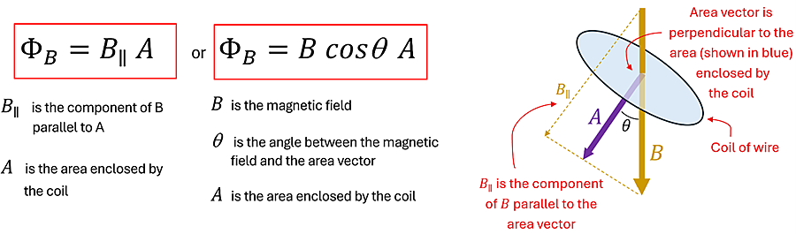
We saw in the previous chapter that an area vector is a vector with a magnitude equal to the surface area enclosed by a loop that points in a direction perpendicular to the surface.  We can see here that B_∥=Bcosθ, where θ  is the angle between the area vector and the direction of the magnetic field.  If B is measured in Tesla and area in square meters, then the calculated flux will be in units of T m² which is defined as a Weber (Wb).

Let’s see how magnetic flux is calculated by considering an example.

Example 1: Calculating Magnetic Flux

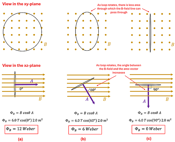
Problem:  A uniform magnetic field of 6.0 T directed out of the page pierces a circular loop of wire of radius 0.80 m.  The loop of wire is in the xy-plane but is allowed to rotate about the y-axis.  Calculate the magnetic flux in each of these situations:

1. In the current configuration
2. If the loop is rotated 60^o
3. If the loop is rotated 90^o

Solution:  To find the magnetic flux, we can begin by finding the area enclosed by the circular loop of wire.  We recall that the area enclosed by this circular loop is given by A= π r² = π(0.80 m)² = 2.0 m² . To help us apply the flux equation for each orientation, a view of both the xy-plane and xz-plane may be helpful.  From the perspective of the xy-plane, we see that as the loop rotates, fewer and fewer magnetic field lines are able to pierce the loop.  From the xz-plane perspective, we see that as the area vector becomes less and less parallel to the direction of the B-field, the flux becomes less and less.  Both are equivalent ways of understanding why the flux is less in (b) and (c) compared to the current configuration (a).  Mathematically, we see that the flux is smaller in (b) and (c) since cos 60^o and cos 90^o is less that the cos 0^o.  

Changing Magnetic Flux

The reason we are so interested in calculating the magnetic flux through the area enclosed by a loop is not so much to determine the magnetic flux at a particular moment in time, but to see how this flux changes over a period of time.  We’ll see in the next section that this ‘rate of change of flux’ is the key to understanding why a current is induced in a wire loop when the magnet is moving near it (and why it does not induce a current when it is stationary). 

So, what could cause the magnetic flux to change?  Since Φ_B=B cosθ A, changing any one of these three variables—B, A, or θ—would change the magnetic flux.  Furthermore, the quicker any one of these quantities changes, the greater the rate of change of magnetic flux. 

Before we link this rate of change of magnetic flux to understanding why this causes a current to be induced in a wire, let’s investigate how changing each of these variables changes the magnetic flux through a loop.

Changing the B-field:  One way to change the magnetic flux is the change the magnitude or direction of the magnetic field.  This could be done by moving the coil closer to or away from a magnet.  This could also be done by changing the current in a wire that is near the loop.  After all, we know that a current-carrying wire produces a B-field; therefore, a changing current would produce a changing B-field and thus a changing flux through the loop.

Example 2: Changing Flux Due to a Moving Magnet

Problem:  The magnetic field of bar magnet along its axis decreases with distance from the magnet itself.  For example, we might approximate that the magnetic field 20 cm away from the north pole of the magnet is 80 µT and 20 µT when it is 40 cm away. 

Imagine a small, circular loop of wire with a radius of 2.0 cm is located at Position 1, a distance of 40.0 cm away from north pole of a magnet as shown.

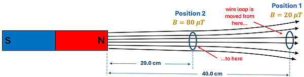
Answer the following questions about this situation:

1. What is the magnetic flux through the circular loop at Position 1?
2. If the loop is moved to Position 2, which is 20.0 cm away from the magnet, what is the flux through the loop now?
3. What is the change in magnetic flux?
4. If moving the loop from Position 1 to Position 2 occurred in 0.80 seconds, what is the average rate of change of magnetic flux?

Solution:  As we did in Example 1, let’s begin by finding the area enclosed by the circular loop.  We find that A=π r² = π (0.020 m)² = 1.26 x 10^-3 m².  Assuming that the magnetic field is uniform across this area and is parallel to the area vector, we can find the answers to (a) and (b) by calculating the flux at Position 1 and Position 2.  For part (c), we just need to subtract the flux at Position 2 from the flux at Position 1.  This gives the change in flux.  Finally, dividing this change in flux by the time over which this change occurred, we can determine the average rate of change of flux.  This is the answer to the last question (d) in the problem. 

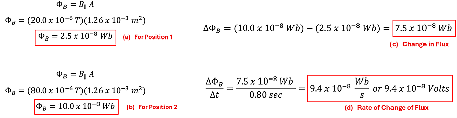
You’ll see in our answer for part (d) that a Weber/sec = Volt.  Why is that?  Didn’t we just learn in the previous section that a change in magnetic flux causes electricity?  The fact that the rate of change of flux has units of Volts is significant.  While uncovering this mysterious connection between magnetism and electricity will become the focus of our exploring Faraday’s Law in the next section,  we can at least start to appreciate why finding the rate of change of flux is an interesting and important calculation to perform. 

Example 3: Changing Flux Due to a Varying Magnetic Field

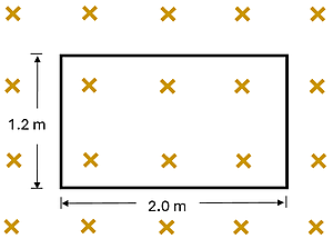
Problem:  A rectangular loop of wire is bathed in is uniform magnetic field across the area enclosed by this loop.  However, this magnetic field varies over time due to a changing current in a nearby solenoid (not shown). The figure on the left shows the dimensions of the loop and the direction of magnetic field a t > 0.  The graph to the right shows the magnitude of the magnetic field as a function of time.

Determine the rate of change of magnetic flux through the loop.

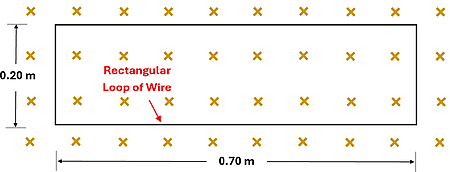
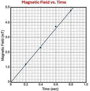
Solution:  We saw above that since Φ_B=B cosθ A, changing any one of these three variables—B, A, or θ —would change the magnetic flux.  We notice here that the direction of the magnetic field is parallel to the area vector.  As a result, the angle between the area vector and the B-field is always 0^o and we know that cos⁡ 0^o = 1. Thus, the angle is not changing.  The area of the loop is not changing either.  The magnetic field, however, is changing.  Thus, the rate of change of magnetic flux is simply the rate of change of the magnetic field time the area enclosed by the loop.  Thus, we can calculate the rate of change of flux like this:

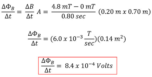
Again, we find it curious that the rate of change of magnetic flux has units of volts.  We have seen in past units that a voltage is responsible for making charges move in a circuit.  Will that be something that happens here?  Before we investigate fully, let’s consider the two other ways that we can change the flux through a loop—changing the area enclosed by the loop and changing the angle that the loop makes with the field.

Example 4: Changing Flux Due to a Changing Area

Let’s focus our attention next on how a changing area will change the magnetic flux through a loop of wire.  Perhaps the most common way that this can occur is by having a loop that moves into or out of a magnetic field.  We’ll consider the example below to illustrate this.

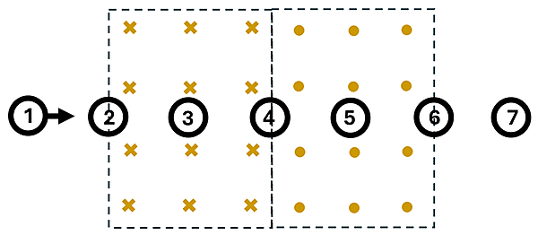
Problem:  Imagine a square loop of wire (2 m x 2 m) entering, traveling through, and then exiting a magnetic field of 2 T that points into the page.  The loop is traveling with a constant velocity of 1 m/s to the right.  The figure below shows the loop’s position at each second.  The shaded region represents the portion of the loop that is in the magnetic field at that moment in time.

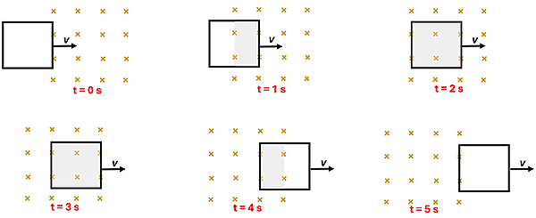
Sketch a graph of (a) the flux vs. time and (b) the change in flux vs. time for the five second interval shown.

Solution:  As the loop enters and exits the magnetic field, we notice that the flux increases and decreases at a constant rate.  This is because the loop is moving at a constant velocity.  When the loop is fully in the magnetic field (from 2-3 seconds), however, the flux is a constant maximum value.  Thus, the change in flux occurs from 0-2 seconds and again from 3-5 seconds.  There is no change in flux from 2-3 seconds.

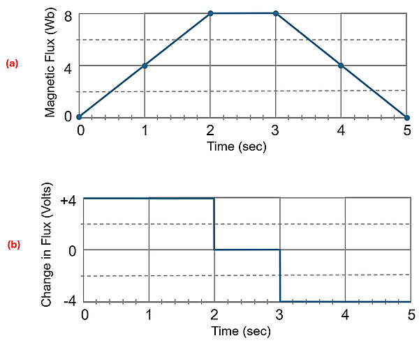
Once again, you might have noticed something pretty interesting.  The slope of the flux vs. time graph is the value of the change in flux at that time.  That makes sense since the rate of change of any quantity is the slope of the graph of that quantity vs time.

Example 5: Changing Flux Due to a Changing Angle

We’ve consider how the flux can change by changing the magnetic field or by changing the area of the loop through which that magnetic field passes.  There is one additional factor in our flux equation, however, and thus one other thing that can change the flux.  If the angle between the magnetic field and the area vector changes, then the flux through the loop will change as well.  We’ll investigate this case by considering a situation similar to the electric motor that we explored in our previous chapter — only this time we will mechanically spin the square loop of wire rather than connecting it to a battery.

Problem: A horseshoe magnetic creates a uniform magnetic field B pointing to the right as shown in the figures below.  A square loop of wire of area A is caused to rotate by a student pushing it so it moves clockwise with a constant angular velocity.  The loop rotates from its orientation in Position A to Position B to Position C over the 2 second interval shown.

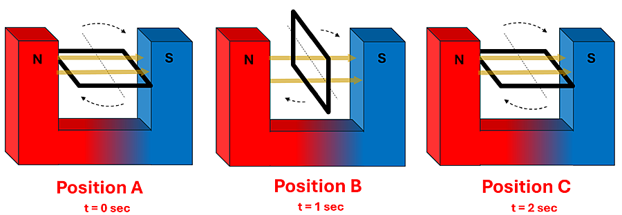
1. During what time interval is the magnetic flux increasing?
2. During what time interval is the magnetic flux decreasing?
3. At what time(s) is the rate of change of flux the greatest?

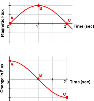
Solution: (a) The flux is increasing from 0 to 1 seconds.  Notice that there is no flux through the loop in Position A and maximum flux in Position B.  Thus, the flux is increasing during the interval from 0 to 1 seconds.  (b) The flux is decreasing from 1 to 2 seconds.  There is a maximum flux through the loop in Position B and the flux continues to decreases as it moves to Position C where there is again no flux.  (c)  The rate of change of flux is greatest at t=0 sec and t=2 sec.  Why is this the case?  The top graph shown to the right illustrates the magnetic flux as a function of time with Positions A, B, and C emphasized.  We learned in the previous example that the slope of the magnetic field vs. time graph is the value of the change in flux at that time.  Notice that the slope of the magnetic flux graph is steepest and a positive value at position A.  We also notice that the slope of the magnetic flux graph at Position B is zero. Finally, the slope at Position C is the largest negative value.  Plotting these slopes on the bottom graph gives us a graph of the change in flux as a function of time. 

Figure 1

In each of the examples above, we’ve investigated both the magnetic flux and the rate of change of flux.  We also found it interesting that this rate of change of magnetic flux has units of Volts. There is a very interesting connection surfacing once again between magnetism and electricity.  We noted in the previous section that a change in magnetism causes electricity.  From this section we can now more precisely state that it is a change in magnetic flux which causes electricity.  How does it cause electricity?  That’s where Faraday's Law comes into play and where we are going next!

Check Your Understanding

Use the following questions to assess your understanding. Tap the Check Answer buttons when ready.

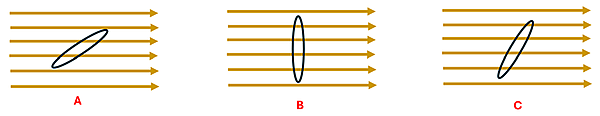
1. The figures below show a side view of the same circular ring in the same magnetic field. The only difference between the figures is the orientation of the ring in the field.  Ranks these in order (greatest to least) of the magnetic flux through the circular ring.

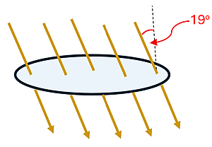
2.  At New York City, the earth’s magnetic field is approximately 5.5 x 10^-5 T and it points more downward than northward.  In fact, the field makes an angle of approximately 19^o from the vertical.  What is the magnetic flux through a basketball hoop (radius = 23 cm) in New York city?  

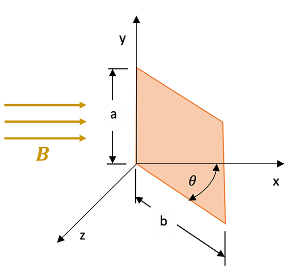
3. A rectangular loop of dimensions a = 2.0 m and b = 3.0 m has one side that runs along the y-axis as shown in the figure.  The bottom side of the loop has been rotated by an angle θ = 30^o from the x-axis.  A uniform magnetic field of B = 0.15 T pointing in the direction of the +x-axis passes through the area enclosed by the loop.  What is the flux through the loop? 

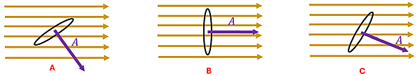
4. A circular loop moves with a constant velocity through two regions where equal magnitude magnetic fields are present.  It first encounters a magnetic field pointing into the page and then out of the page as shown.

Rank the magnitude of the rate of change of flux (from greatest to least) for each of the positions shown.  If some values are the same, group them with parenthesis (such as 1, (2, 3), 4).

5. A time-varying magnetic field varies according to the equation B(t) = B_o – Ct, where B(t) is the magnetic field at time t, B_o = 1.4 T, and C = 0.2 T/sec.   A rectangular loop is placed in this field as shown.  Determine each of the following:

1. Magnetic flux at t = 0 seconds
2. Magnet flux at t = 7 seconds
3. Change in magnetic flux from 0 to 7 seconds
4. Rate of change of magnetic flux during this interval of time

 
Figure 1 Modified from: https://commons.wikimedia.org/w/index.php?search=sine+and+cosine+graphs&title=Special:MediaSearch&type=image and https://commons.wikimedia.org/w/index.php?search=sine+and+cosine+graphs&title=Special:MediaSearch&type=image