Position-Velocity-Acceleration - Complete Toolkit
Objectives
-
Students should understand the difference between the terms distance and displacement, speed and velocity, and velocity and acceleration.
-
Students should combine an understanding of these terms with the use of pictorial representations (dot diagrams, vector diagrams) and data representations (position-time and velocity-time data) in order to describe an object’s motion in one dimension.
-
Students should relate the distance, displacement, average speed, average velocity, change in velocity, time and acceleration to each other in order to solve word problems.
Readings from The Physics Classroom Tutorial
-
The Physics Classroom Tutorial, 1D-Kinematics Chapter, Lesson 1
http://www.physicsclassroom.com/class/1DKin/Lesson-1/Introduction
Interactive Simulations
-
Graph Matching Motion Model Simulation
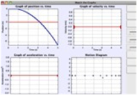 Powerful way to investigate the meaning of shape and slope for 3 types of motion graphs. To set it up correctly requires the student to analyze and interpret computer-generated motion of a blue object moving either with constant velocity or constant acceleration. Next, match the motion by using sliders to set initial position, velocity, and acceleration of an adjacent red object. Last, use sliders to predict the shape of the related velocity and acceleration graphs to give correct straight-line slopes.
Video and Animations
-
Physlet Physics: Position and Displacement Interactive Animation
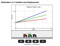 Short activity lets students compare the animated motion of three Monster trucks. In the first animation, the trucks start at different positions but travel at the same average speed. In the second, the trucks’ initial positions are the same but each truck travels a different distance and displacement. The animations are intended to help students recognize and differentiate Distance vs. Time and Displacement vs. Time.
-
Georgia Public Broadcasting: Physics 301 – Analysis of Motion Video (30 minutes)
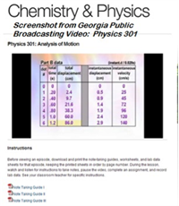 Good choice for flipped lesson – this 30-minute video takes students through the basics of 1-D motion, from displacement through velocity and acceleration. Teachers: it includes detailed procedures for doing a motion experiment using ticker tape. It also provides note-taking guides, worksheets, and data tables tailored specifically for use while watching the video. Free teacher materials can be requested and, to ensure security, will be mailed directly to the school district. This is a solid way to bridge learning gaps for students with reading disabilities or kids who are struggling with concepts of kinematics.
Labs and Investigations
Minds On Physics Internet Modules:
The Minds On Physics Internet Modules are a collection of interactive questioning modules that target a student’s conceptual understanding. Each question is accompanied by detailed help that addresses the various components of the question.
-
Kinematic Concepts module, Assignment KC2 - Distance vs. Displacement
-
Kinematic Concepts module, Assignment KC3 – Speed vs. Velocity
-
Kinematic Concepts module, Assignment KC4 – Acceleration
-
Kinematic Concepts module, Assignment KC5 – Oil Drop Representations
-
Kinematic Concepts module, Assignment KC8 – Pos-time and Vel-time Data Analysis
Concept Building Exercises:
-
The Curriculum Corner, Describing Motion Verbally with Distance and Displacement
-
The Curriculum Corner, Describing Motion Verbally with Speed and Velocity
-
The Curriculum Corner, Acceleration
-
The Curriculum Corner, Describing Motion with Diagrams
-
The Curriculum Corner, Describing Motion Numerically
Problem-Solving Exercises:
-
The Calculator Pad, ChapterGoesHere, Problems #1-9
Science Reasoning Activities:
-
Science Reasoning Resource CD, 1D Kinematics, Stopping Distance
Common Misconceptions:
-
Confusion of Speed and Acceleration
Students commonly confuse the idea of accelerating as meaning to go fast. Emphasize that accelerating objects are not moving fast, but rather changing how fast they are moving (and/or what direction they are moving).
-
The Use of + and – to Describe Direction
It is a common convention to use + and – signs to describe the direction of velocity and acceleration. The convention is borrowed from mathematics in which the – region of a graph or number line is left or below the origin. As such, negative signs are used to describe vectors that have a leftward or a downward direction. This usage unfortunately leads to incorrect beliefs such as an object with a velocity of -20 m/s is moving slower than an object with a velocity of -5 m/s since the number -20 is less than (more negative than) -5. The proper approach to this is to translate “a velocity of -20 m/s” to mean “an object moving to the left with a speed of 20 m/s.”
-
Confusion about the Direction of Velocity and Acceleration
It is common for students to incorrectly believe that the direction of the acceleration is in the same direction that an object is moving. This is only true of objects that are speeding up. For objects that are slowing down, the acceleration is directed in a direction that is opposite of the object’s motion.
Related PER (Physics Education Research)
-
Kinematics Graph Interpretation Project
http://www.ncsu.edu/ncsu/pams/physics/Physics_Ed/TUGK.html
Recent work has uncovered a consistent set of student difficulties with graphs of position, velocity, and acceleration vs. time. For the busy teacher, this synopsis will be a quick read but worth every minute. It organizes the findings of several years of the Kinematics Graph Interpretation Project on one page.
-
Searching for Evidence of Student Understanding, T. Bartiromo, presented at the Physics Education Research Conference 2010, Portland, Oregon
http://www.compadre.org/per/items/detail.cfm?ID=10390
This research examined whether high school students can translate between representations (an ability often considered to be an “expert trait” in solving physics problems). It also gauged whether requiring multiple representations for a single problem helped instructors better assess student understanding. It’s a short read (3.5 pages), and has interesting implications: “We can argue that by assessing students with multiple choice questions or by requiring only one representation, one might get a false sense of students’ mastery…..Therefore, assessments need to include problems in which students respond with more than one representation.”
Standards:
A. Next Generation Science Standards (NGSS)
Note: The topic of kinematics is not directly covered in the NGSS.
B. Common Core Standards for Mathematics – Grades 9-12
Standards for Mathematical Practice
-
MP.2 Reason abstractly and quantitatively
-
MP.6 Attend to precision
-
MP.8 Look for and express regularity in repeated reasoning
Quantities: Reason Quantitatively and Use Units to Solve Problems
-
N-Q.1 Use units as a way to understand problems and to guide the solution of multi-step problems; choose and interpret units consistently in formulas; choose and interpret the scale and the origin in graphs and data displays.
-
N-Q.3 Choose a level of accuracy appropriate to limitations on measurement when reporting quantities.
Algebra: Seeing Structure in Expressions – Interpret the Structure of Expressions
-
A-SSE.1.a Interpret parts of an expression, such as terms, factors, and coefficients
-
A-SSE.2 Use the structure of an expression to identify ways to rewrite it.
Algebra: Creating Equations
-
A-CED.2 Create equations in two or more variables to represent relationships between quantities; graph equations on coordinate axes with labels and scales.
-
A-CED.4 Rearrange formulas to highlight a quantity of interest, using the same reasoning as in solving equations.
Functions: Interpret Functions that Arise in Terms of a Context
-
F-IF.4 For a function that models a relationship between two quantities, interpret key features of graphs and tables in terms of the quantities, and sketch graphs showing key features given a verbal description of the relationship.
-
F-IF.6 Calculate and interpret the average rate of change of a function (presented symbolically or as a table) over a specified interval. Estimate the rate of change from a graph.
Functions: Analyze Functions Using Different Representations
-
F-IF.7.a Graph linear and quadratic functions and show intercepts, maxima, and minima.
Building Functions: Linear, Quadratic, and Exponential Models
-
F-LE.1.b Recognize situations in which one quantity changes at a constant rate per unit interval relative to another.
-
F-LE.1.c Recognize situations in which a quantity grows or decays by a constant percent rate per unit interval relative to another.
Functions: Interpret Expressions for Functions in Terms of the Situation They Model
-
F-LE.5 Interpret the parameters in a linear or exponential function in terms of a context.
Reading Level
This set of tutorials scored 48.94 on the Flesch-Kincaid Readability Index, corresponding to Grade 10. It scored 12.28 on the Gunning-Fog Index, which indicates the number of years of formal education a person requires in order to easily understand the text on the first reading (corresponding to Grade 12).
C. Common Core Standards for English/Language Arts (ELA) – Grades 9-12
Key Ideas and Details: High School
-
RST.11-12.2 Determine the central ideas or conclusions of a text; summarize complex concepts, processes, or information presented in a text by paraphrasing them in simpler but still accurate terms.
Craft and Structure – High School
-
RST.11-12.4 Determine the meaning of symbols, key terms, and other domain-specific words and phrases as they are used in a specific scientific or technical context relevant to grades 11-12 texts and topics.
Integration of Knowledge and Ideas – High School
-
RST.11-12.9 Synthesize information from a range of sources (e.g., texts, experiments, simulations) into a coherent understanding of a process, phenomenon, or concept, resolving conflicting information when possible.
Range of Reading and Level of Text Complexity – High School
-
RST.11.12.10 By the end of grade 12, read and comprehend science/technical texts in the grades 11-CCR text complexity band independently and proficiently.
D. College Ready Physics Standards (Heller and Stewart)
Essential Knowledge-Middle School
Constant and Changing Linear Motion
-
M.3.1.1 The basic patterns of the straight-line motion of objects are: no motion, moving with a constant speed, speeding up, slowing down and changing (reversing) direction of motion. Sometimes an object’s motion can be described as a repetition and/or combination of the basic patterns of motion.
-
M.3.1.2 An object that travels the same distance in each successive unit of time has a constant speed. The constant speed of an object can be represented by and calculated from the mathematical representation (speed = distance traveled/time interval), data tables, a motion diagram, and the slope of the linear distance versus time graph.
-
M.3.1.3 When the distance an object travels increases with each successive unit of time, it is speeding up; when the distance an object travels decreases with each successive unit of time, it is slowing down.
-
M.3.1.4 The relationship between distance and time is nonlinear when an object’s speed is changing and when it is moving in a series with different constant speeds.
-
The constant speed an object would travel to move the same distance in the same total time interval is the average speed.
-
Average speed can be represented and calculated from the mathematical representation (average speed – total distance traveled/total time interval), data tables, and the nonlinear Distance vs. Time graph.
-
For objects traveling to a final destination in a series of different constant speeds, the average speed is not the same as the average of the constant speeds.
Essential Knowledge: High School
Constant and Changing Linear Motion
-
H.3.1.1 The displacement, or change in position, of an object is a vector quantity that can be calculated by subtracting the initial position from the final position, where initial and final positions can have positive and negative values. Displacement is not always equal to the distance traveled.
-
H.3.1.2 An object that travels the same displacement in each successive unit time interval has constant velocity. Constant velocity is a vector quantity and can be represented by and calculated from a position versus time graph, a motion diagram or the mathematical representation for average velocity. The sign (+ or -) of the constant velocity indicates the direction of the velocity vector, which is the direction of motion.
-
H.3.1.3 The constant velocity an object would travel to achieve the same change in position in the same time interval, even when the object’s velocity is changing, is the average velocity for the time interval. Average velocity can be mathematically represented by vave = (xf - xi)/(tf - ti). For straight-line motion, average velocity can be represented by and calculated from the mathematical representation, a curved position versus time graph and a motion diagram.
-
H.3.1.4 The velocity of an object in straight-line motion changes continuously, from instant to instant while it is speeding up or slowing down and/or changing direction. The velocity of an object at any instant (clock reading) is called its instantaneous velocity. The object does not have this velocity over any time interval or travel any distance with this velocity. Instead, the instantaneous velocity is the constant velocity at which an object would continue to move if its motion stopped changing at that instant. An object with zero instantaneous velocity can be accelerating (e.g., motion up a ramp then back down the ramp).
-
H.3.1.5 When the change in an object’s instantaneous velocity is the same in each successive unit time interval, the object has constant acceleration. For straight-line motion, constant acceleration can be represented by and calculated from a linear instantaneous velocity versus time graph, a motion diagram and the mathematical representation [a = (vf - vi)/(tf - ti)]. The sign (+ or -) of the constant acceleration indicates the direction of the change-of-velocity vector. A negative sign does not necessarily mean that the object is traveling in the negative direction or that it is slowing down. [BOUNDARY: The term “deceleration” should be avoided because students tend to associate a negative sign of acceleration only with slowing down.]
Learning Outcomes
-
Represent and calculate the distance traveled by an object, as well as the displacement, the speed and the velocity of an object for different problems. Representations include data tables, distance versus time graphs, position versus time graphs, motion diagrams and their mathematical representations. Interpret the meaning of the sign (+ or -) of the displacement and velocity.
-
Investigate, and make a claim about the straight-line motion of an object in different laboratory situations. Representations include data tables, position versus time graphs, instantaneous velocity versus time graphs, motion diagrams, and their mathematical representations. When appropriate, calculate the constant velocity, average velocity or constant acceleration of the object. Interpret the meaning of the sign of the constant velocity, average velocity or constant acceleration. Interpret the meaning of the average velocity.
-
Explain what is “constant” when an object is moving with a constant velocity and how an object with a negative constant velocity is moving. Justify the explanation by constructing sketches of motion diagrams and using the shape of position and instantaneous velocity versus time graphs.
-
Explain what is “constant” when an object is moving with a constant acceleration, and explain the two ways in which an object that has a positive constant acceleration and a negative constant acceleration. Justify the explanations by constructing sketches of motion diagrams and using the shape of instantaneous velocity versus time graphs.
-
Compare and contrast the following: distance traveled and displacement; speed and velocity; constant velocity and instantaneous velocity; constant velocity and average velocity; and velocity and acceleration.
-
Translate between different representations of the motion of objects: verbal and/or written descriptions, motion diagrams, data tables, graphical representations (position versus time graphs and instantaneous velocity versus time graphs) and mathematical representations.