Chapter 9: Rotation and Balance - Lesson 1: Rotational Kinematics
Equations of Rotational Kinematics
Hold down the T key for 3 seconds to activate the audio accessibility mode, at which point you can click the K key to pause and resume audio. Useful for the Check Your Understanding and See Answers.
The BIG 4 Equations for Rotational Motion
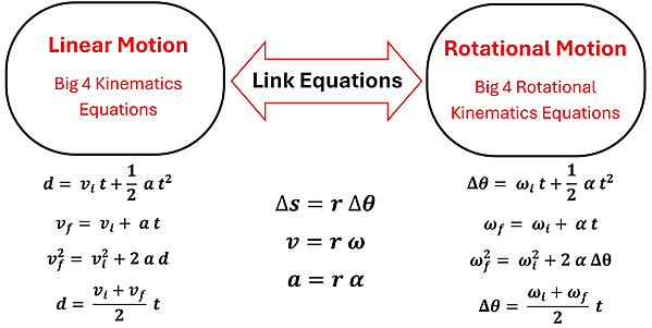
When we learned the big four kinematics equations back in 1-D Kinematics, we saw their power in solving constant acceleration motion problems. As you might expect, we can do the same with the big four equations for rotational motion. Even better, you may be able to predict the big four equations for rotational motion by recalling that each translational quantity (d, v, and a) has its rotational counterpart (∆θ, ω, and ⍺). By simply substituting the rotational quantity for the translational quantity, we have the big four kinematics equations for rotation!
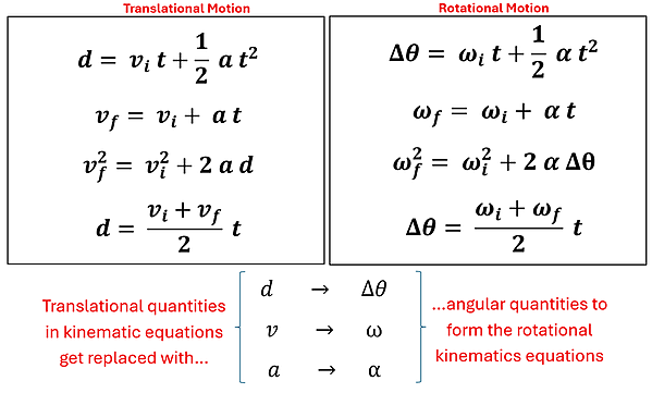
There was one assumption that we made when we introduced the big four kinematics equations. We assumed that we were studying motion with constant acceleration. That means that an object speeds up or slows down at the same rate each second. (Constant accelerated motion includes motion with no acceleration, as the acceleration would be constant at 0 m/s2.) It follows, then, that our big four equations for rotation motion require a similar assumption. These equations will help us solve rotation motion problems with constant angular acceleration. We'll limit our problems to situations that meet this requirement.
Problem-Solving Strategy Revisited
Whenever we solve physics problems—and especially kinematics problems—having a strategy is important. Let's revisit the same problem-solving approach we used in Lesson 6 of 1-D Kinematics. It was a good strategy then, and it's just as helpful now.
We begin by drawing a diagram and then making a list of the givens and the unknown we are trying to find. This will often lead us to the equation we'll need to use. We will then substitute our values, solve, and then check our answer to make sure it seems reasonable.
Ready to give this a try? Let's see if we can solve a couple of rotational motion problems using our new big four equations and our tried-and-true problem-solving strategy.
Problem-Solving Strategy
- Construct an informative diagram of the physical situation.
- Identify and list the given information in variable form.
- Identify the list of unknown information in variable form.
- Identify and list the equation that will be used to determine unknown information from known information
- Substitute known values into the equation and use appropriate algebraic steps to solve for the unknown information.
- Check your answer to ensure that it is reasonble and mathematically correct.
Example 1: Music to My Ears
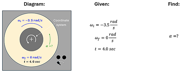
Problem: Iwona Listen has an old phonograph turntable that spins her records at 3.5 rad/sec in the clockwise direction. The device slows down and stops 4.0 seconds after turning it off. What is the angular acceleration of her record as it slows to a stop?
Solution: Let's begin with a diagram of Iwona's turntable. We'll include a coordinate system on our diagram. Since we usually call counterclockwise (CCW) the positive direction, we'll label this as our coordinate system. Next, we'll make a list of the givens and the unknown we are trying to find. Three pieces of information are given: ωi, ωf, and t. We've labeled ωi as negative since the record is rotating in the clockwise (CW) direction. ωf is zero since the record comes to rest. The time is also given. Finally, the unknown we are trying to find is the angular acceleration α. We'll label this under the "Find" column.
Only one of our big four rotational kinematics equations has these given/unknown variables in it. That's how we know to pick the equation:
ωf = ωi + α t
We'll now solve this equation algebraically for the variable that we are trying to find, substitute values, and solve…
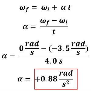
It makes sense that we get a positive (CCW) angular acceleration since the record is slowing down while traveling in the negative (CW) direction.
Example 2: Round and Round We Go
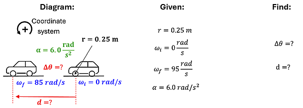
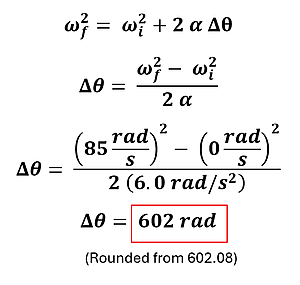
Problem: Benna Round tested out her new tires when she stepped on the gas as the light turned green. The 0.25 m radius tires on her car went from having an angular velocity of 0 rad/s to 85 rad/s as they experienced an angular acceleration of 6.0 rad/s2.
(A) Through what angle did the wheels turn?
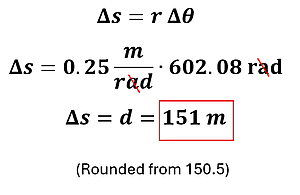
(B) What distance did her car travel?
Solution: We'll start by making a diagram to visualize the situation. We've again included a coordinate system to show that we're defining CCW as the positive direction. We've also identified the givens and labeled what we are trying to find.
For part (a), we see that our third rotational kinematics equation includes ωi, ωf, ⍺, and ∆θ. (We won't need r yet; we'll save this for the part of the problem where we solve for the distance d.) Solving this algebraically for ∆θ, substituting values, and then simplifying shows us that her tires turned through 602 radians (nearly 96 rotations of the tires).
For part (b), we'll use our first link equation from the previous section of this lesson. We can solve for ∆s in this equation, which is the total distance around and around the circumference of the tires if you continue rotating through 602 radians. Do you see that d and ∆s are interchangeable? It's true that the ∆s we solved for is the same as the distance d the car will have traveled down the road!
Conclusion
The big four kinematics equations from 1-D Kinematics allow us to perform calculations involving the translational quantities of d, v, and a. The big four rotational kinematics equations that we just learned allow us to perform calculations involving ∆θ, ω, and ⍺. It is link equations from the previous part of this lesson, however, that allow us to connect these—giving us even greater problem-solving power as we study the motion of something like a car that has both linear and rotational motion!
Check Your Understanding
Use the following questions to assess your understanding. Tap the Check Answer buttons when ready.
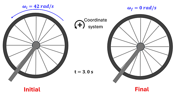
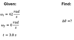
1. A bicycle is turned upside down and the wheel is spun while the owner adjusts the brakes. With the wheels spinning at 42 rad/s, the brakes are applied, and it takes 3.0 seconds for the wheel to come to rest. How many rotations did the wheel make during this braking process?
(A) On paper, make a sketch to help visualize this situation.
(B) Identify the givens and the unknown you are trying to find.
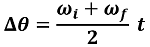
(C) Of the four rotational kinematics equations, which one will you use?
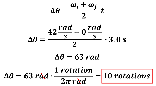
(D) Substitute in values and solve for rotations of the wheel.
(E) Does this answer make sense?
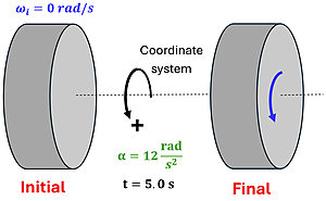
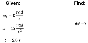
2. The motor of a grinding wheel in a machine shop causes the wheel to experience an average angular acceleration of 12 rad/s2 when it is turned on. If it takes 5.0 seconds to get up to its full speed, through what angle (in radians) did the wheel spin on startup?
(A) On paper, make a sketch to help visualize this situation.
(B) Identify the givens and the unknown you are trying to find.
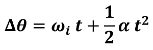
(C) Of the four rotational kinematics equations, which one will you use?
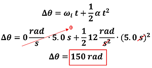
(D) Substitute in values and solve for the angle through which the wheel travels on startup.
(E) Does this answer make sense?
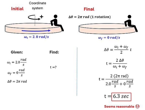
3. A merry-go-round at the neighborhood park is spinning at 2.0 rad/s. To bring the merry-go-round to rest, a child drags her feet on the ground and stops it after it makes exactly one rotation. For how much time was the child dragging her feet? Use the problem-solving strategy as you work through this problem and then check your work.
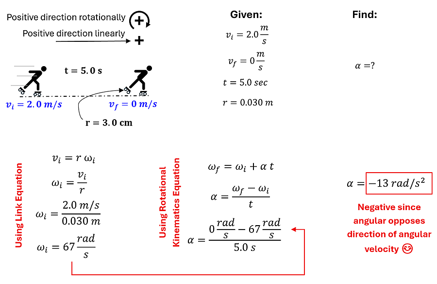
4. A rollerblader travels at 2.0 m/s when he encounters a rough patch of pavement and eventually coasts to a stop in 5.0 seconds. The diameter of a rollerblade wheel is 6.0 cm. What was the angular acceleration of the rollerblade wheels (in rad/s2)? (Here you will need to not only use one of the big four rotational kinematics equations, but you'll need to employ one of the link equations from the previous section as well.)
Looking for additional practice? Check out the CalcPad for additional practice problems (RK5, RK6, RK7 and RK8).